Fitting and Statistics¶

Warning

pytc will fit all sorts of complicated models to your data. It is up to you to make sure the fit is justified by the data. You should always follow best practices for selecting the your model (choosing the simplest model, inspecting residuals, knowing the assumptions made, etc.)

Fits¶

pytc implements a variety of fitting strategies:

BayesianFitter uses Markov-Chain Monte Carlo to estimate posterior probability distributions for all fit parameters. (Recommended)
BootstrapFitter samples from uncertainty in each heat and then fits the model to pseudoreplicates using unweighted least-squares regression.
MLFitter fits the model to the data using least-squares regression weighted by the uncertainty in each heat. (Default)

Details on these strategies and their implementation below.

Fit Results¶

After you have peformed the fit, there are a variety of ways to access and assess your results. These are available for all fit strategies.

Parameter estimates as csv¶

g.fit_as_csv

where g is a GlobalFit instance. This will print something like:

# Fit successful? True
# 2017-05-13 09:27:25.177062
# Fit type: maximum likelihood
# AIC: -96.23759423779696
# AICc: -93.8028116291013
# BIC: -84.30368995841131
# F: 292708.2585218862
# Rsq: 0.9999672039142115
# Rsq_adjusted: 0.9999637876552752
# ln(L): 54.11879711889848
# num_obs: 54
# num_param: 5
# p: 1.1102230246251565e-16
type,name,exp_file,value,stdev,bot95,top95,fixed,guess,lower_bound,upper_bound
local,dilution_heat,ca-edta/tris-01.DH,1.15715e+03,4.65377e+02,2.21447e+02,2.09285e+03,False,0.00000e+00,-inf,inf
local,K,ca-edta/tris-01.DH,4.05476e+07,4.31258e+05,3.96805e+07,4.14147e+07,False,1.00000e+06,-inf,inf
local,dilution_intercept,ca-edta/tris-01.DH,-6.12671e-01,6.71064e-02,-7.47597e-01,-4.77744e-01,False,0.00000e+00,-inf,inf
local,dH,ca-edta/tris-01.DH,-1.15669e+04,1.00638e+01,-1.15872e+04,-1.15467e+04,False,-4.00000e+03,-inf,inf
local,fx_competent,ca-edta/tris-01.DH,9.73948e-01,8.86443e-05,9.73770e-01,9.74126e-01,False,1.00000e+00,-inf,inf

Lines starting with “#” are statistics and fit meta data. The statistical output is described in the statistics section below. Rendered as a table, the comma- separated output has the following form:

type	name	exp_file	value	stdev	bot95	top95	fixed	guess	lower_bound	upper_bound
local	dilution_heat	ca-edta/tris-01.DH	1.15715e+03	4.65377e+02	2.21447e+02	2.09285e+03	False	0.00000e+00	-inf	inf
local	K	ca-edta/tris-01.DH	4.05476e+07	4.31258e+05	3.96805e+07	4.14147e+07	False	1.00000e+06	-inf	inf
local	dilution_intercept	ca-edta/tris-01.DH	-6.12671e-01	6.71064e-02	-7.47597e-01	-4.77744e-01	False	0.00000e+00	-inf	inf
local	dH	ca-edta/tris-01.DH	-1.15669e+04	1.00638e+01	-1.15872e+04	-1.15467e+04	False	-4.00000e+03	-inf	inf
local	fx_competent	ca-edta/tris-01.DH	9.73948e-01	8.86443e-05	9.73770e-01	9.74126e-01	False	1.00000e+00	-inf	inf

type: “local” or “global”
name: parameter name
exp_file: name of experiment file
value: estimate of the parameter
stdev: standard deviation of parameter estimate
bot95/top95: 95% confidence intervals of parameter estimate
fixed: “True” or “False” depending on whether parameter was held to fixed value
guess: parameter guess
lower_bound/upper_bound: bounds set on the fit parameter during the fit

Fit and residuals plot¶

g.plot()

where g is a GlobalFit instance. This will create something like:

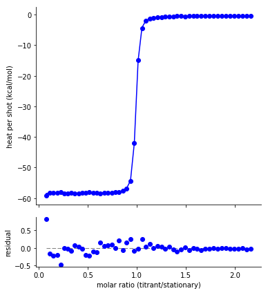
The fit residuals should be randomly distributed around zero, without systematic deviations above or below. Non-random residuals can indicate that the model does not adequately describe the data, despite potentially having a small residual standard error.

Corner plots¶

One powerful way to assess the fit results is through a corner plot, which shows the confidence on each fit parameter, as well as covariation between each parameter. The quality of the histograms is also an indication of whether you have adequate sampling when using the bootstrap or bayesian methods.

g.corner_plot()

where g is a GlobalFit instance. This will create something like:

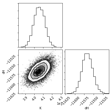
The diagonal shows a histogram for that parameter. The bottom-left cells show a 2D histogram of covariation between those parameters.

g.plot_corner uses keywords to find and filter out nuisance parameters like fx_competent or dilution_heat. To see these (or modify the filtering) change the filter_params list passed to the function.

Statistics¶

g.fit_stats

where g is a GlobalFit instance. This will return a dictionary of fit statistics with the following keys.

AIC: Akaike Information Criterion
AICc: Akaike Information Criterion corrected for finite sample size
BIC: Bayesian Information Criterion
df: degrees of freedom
F: The F test statistic
ln(L): log likelihood of the model
num_obs: number of data points
num_param: number of floating parameters fit
Rsq: \(R^{2}\)
Rsq_adjusted: \(R^{2}_{adjusted}\)
Fit type: the type of fit (maxium likelihood, bootstrap, or bayesian)
Keys like ” bayesian: num_steps” provide information specific to a given fit type.

Model comparison¶

Models with more parameters will generally fit the data better than models with fewer parameters. These extra parameters may or may not be meaningful. (You could, for example, fit \(N\) data points with \(N\) parameters. This would give a perfect fit – and very little insight into the system). A standard approach in model fittng is to choose the simplest model consistent with the data. A variety of statistics can be used to balance fitting the data well against the addition of many parameters. pytc returns four test statistics that penalize models based on the number of free parameters: Akaike Information, corrected Akaike Information, Bayesian Information, and the F-statistic.

The pytc.util.compare_models function will conveniently compare a collection of models, weighting them by AIC, AICc, and BIC.

Fitting Strategies¶

pytc implements multiple fitting strategies including least-squares regression, bootstrap sampling + least squares, and Bayesian MCMC. These are implemented as subclasses of the pytc.fitters.Fitter. base class.

Bayesian¶

pytc.fitters.BayesianFitter.

Uses Markov-Chain Monte Carlo (MCMC) to sample from the posterior probability distributions of fit parameters. pytc uses the package emcee to do the sampling. The log likelihood function is:

\[ln(L) = -0.5 \sum_{i=0}^{i < N} \Big [ \frac{(dQ_{obs,i} - dQ_{calc,i}(\vec{\theta}))^{2}}{\sigma_{i}^{2}} + ln(\sigma_{i}^{2}) \Big ]\]

where \(dQ_{obs,i}\) is an observed heat for a shot, \(dQ_{calc,i}\) is the heat calculated for that shot by the model, and \(\sigma_{i}\) is the experimental uncertainty on that heat.

The prior distribution is uniform within the specified parameter bounds. If any parameter is outside of its bounds, the prior is \(-\infty\). Otherwise, the prior is 0.0 (uniform).

The posterior probability is given by the sum of the log prior and log likelihood functions.

\[ln(P) = ln(L) + ln(prior)\]

Parameter estimates¶

Parameter estimates are the means of posterior probability distributions.

Parameter uncertainty¶

Parameter uncertainties are estimated by numerically integrating the posterior probability distributions.

Bootstrap¶

pytc.fitters.BootstrapFitter.

Samples from experimental uncertainty in each heat and then peforms unweighted least-squares regression on each pseudoreplicate using scipy.optimize.least_squares. The residuals function is:

\[\vec{r} = \vec{dQ}_{obs} - \vec{dQ}_{calc}(\vec{\theta})\]

where \(\vec{dQ}_{obs}\) is a vector of the observed heats and \(\vec{dQ}_{calc}(\vec{\theta})\) is a vector of heats observed with fit paramters \(\vec{\theta}\).

This uses the robust Trust Region Reflective method for the nonlinear regression.

Parameter estimates¶

Parameter estimates are the means of bootstrap pseudoreplicate distributions.

Parameter uncertainty¶

Parameter uncertainties are estimated by numerically integrating the bootstrap pseudoreplicate distributions.

Least-squares regression¶

pytc.fitters.MLFitter.

Weighted least-squares regression using scipy.optimize.least_squares. The residuals function is:

\[\vec{r} = \frac{\vec{dQ}_{obs} - \vec{dQ}_{calc}(\vec{\theta})}{\vec{\sigma}_{obs}}\]

where \(\vec{dQ}_{obs}\) is a vector of the observed heats, \(\vec{dQ}_{calc}(\vec{\theta})\) is a vector of heats observed with fit paramters \(\vec{\theta}\), and \(\vec{\sigma}_{obs}\) are the uncertainties on each fit.

This uses the robust Trust Region Reflective method for the nonlinear regression.

Parameter estimates¶

The parameter estimates are the maximum-likelihood parameters returned by scipy.optimize.least_squares.

Parameter uncertainty¶

We first approximate the covariance matrix \(\Sigma\) from the Jacobian matrix \(J\) estimated by scipy.optimize.least_squares:

\[\Sigma \approx [2(J^{T} \cdot J)]^{-1}\]

We can then determine the standard deviation on the parameter estimates \(\sigma\) by taking the square-root of the diagonal of \(\Sigma\):

\[\sigma = \sqrt(diag(\Sigma))\]

Ninety-five percent confidence intervals are estimated using the Z-score assuming a normal parameter distribution with the mean and standard deviations determined above.

Warning

Going from \(J\) to \(\Sigma\) is an approximation. This is susceptible to numerical problems and may not always be reliable. Use common sense on your fit errors or, better yet, do Bayesian integration!